Assignment
Acoustic Analogies
Problem description
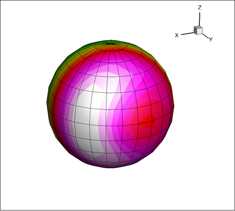
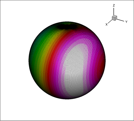
Within an artificial boundary in the form of a sphere with radius R=1 m, centered at (0,0,0), there are some unknown noise sources due to unsteady flow. On the surface of the sphere and outside the sphere the average flow velocity is considered to be zero and the average pressure and density are constant. Acoustic quantities such as fluctuations of density, velocity and pressure are measured on the surface of the sphere. Data in the form of geometry and acoustics can be found using the listed links below.
In the geometry files the following information is given:
NI NJ
XC YC ZC SXN SYN SZN SL
.
.
.
XC YC ZC SXN SYN SZN SL
where NI is the number of panels in longitudinal direction and NJ the corresponding number in latitudinal direction (I is in inner loop, J is in outer loop). For each surface panel XC,YC,ZC are the coordinates of the panel centroid, SXN,SYN,SZN are the coordinates of the outward facing unit normal vector, and SL is the surface area. In the acoustic data files the following data is given:
NT
T
ROP UP VP WP PP DPPN DPPT
.
.
.
ROP UP VP WP PP DPPN DPPT
.
.
.
.
.
.
.
T
ROP UP VP WP PP DPPN DPPT
.
.
.
ROP UP VP WP PP DPPN DPPT
In this case NT is the number of time steps, T is the time for a batch of data that follows, ROP, UP, VP, WP, PP are the acoustic fluctuations of density, velocity components and pressure, DPPN is the gradient of PP in the normal direction and DPPT is the time derivative of PP. Note that the data is periodic, i.e. the fluctuations for the last time are identical to the fluctuations for the first time. The data for a given time is ordered in the same manner as the surface panels in the geometric data file.
Assignments
The assignments are as follows (you need only do one of them):
| Assignment 1 |
| Use the data to compute the pressure signal at the observer positions (1,1,1), (3,3,3) and (10,10,10), for observer time t=0-0.005 s, in steps of 0.00025 s. Choose Kirchhoff’s method with observer time approach for the computations. The reference density is 1.2 kg/m3, the reference speed of sound is 340 m/s. Do this for all four surface discretizations if possible. |
| Assignment 2 |
| Use the data to compute the pressure signal at the observer positions (1,1,1), (3,3,3) and (10,10,10), for observer time t=0-0.005 s, in steps of 0.00025 s. Choose Kirchhoff’s method with source time approach for the computations. The reference density is 1.2 kg/m3, the reference speed of sound is 340 m/s. Do this for all four surface discretizations if possible. |
| Assignment 3 |
| Use the data to compute the pressure signal at the observer positions (1,1,1), (3,3,3) and (10,10,10), for observer time t=0-0.005 s, in steps of 0.00025 s. Choose FWH’s method for stationary permeable surface with the observer time approach for the computations. The reference density is 1.2 kg/m3, the reference speed of sound is 340 m/s. Do this for all four surface discretizations if possible. |
The assignments may be solved either by MATLAB or by coding in some computer language, e.g. FORTRAN, C, JAVA, C++, python, etc.
Questions on lecture material to be answered in writing
| Problem 1 |
| An engineer sitting in an office complains about ventilation noise. Air is forced into the room from an air vent close to the ceiling. The air comes from an extensive duct system with many junctions, mesh filters and fans. The engineer tries to analyze the noise and reaches the conclusion that it consists of both tonal noise and broadband noise, in a wide frequency band. However, since the engineer knows very little about aero-acoustics, he or she needs some help in formulating possible noise sources. Describe some possible noise sources and also how the generated noise may be affected while propagating through the duct system into the room. You may exclude all effects due to vibrations of the duct walls. |
| Problem 2 |
| A sound source that moves with a constant velocity through air at rest will generate noise that differs from that of a stationary source. Describe in which way the movement of the source affects the noise perceived by a stationary observer. |
| Problem 3 |
| The sound field generated by a stationary monopole in air at rest, with a harmonic time variation (sinusoidal signal), is given by the formulas below: $$p^\prime({\mathbf{x}},t)=\frac{A}{4\pi R}\cos\left[\omega\left(t-\frac{R}{c_o}\right)\right]$$ $${\mathbf{u}}^\prime({\mathbf{x}},t)=\frac{A({\mathbf{x}}-{\mathbf{x}}_S)}{4\pi \rho_o\omega R^3}\sin\left[\omega\left(t-\frac{R}{c_o}\right)\right]+ \frac{A({\mathbf{x}}-{\mathbf{x}}_S)}{4\pi \rho_o c_o R^2}\cos\left[\omega\left(t-\frac{R}{c_o}\right)\right]$$ $$\rho^\prime({\mathbf{x}},t)=\frac{1}{c_o^2}p^\prime({\mathbf{x}},t)$$ where $$R=\left|{\mathbf{x}}-{\mathbf{x}}_S\right|$$ By looking at these expressions it is possible to distinguish between near-field and far-field sound terms. Which is which? Write down the motivation for your choice. Compare the far-field noise from the monopole with that of a planar sound wave. In what way are they similar/different? |
| Problem 4 |
| When the sound source and observer are both moving through the air (with the same speed and direction), we refer to this as the ‘wind tunnel scenario’. A simple Galileo transformation gives us instead a stationary source and a stationary observer, both immersed in a uniform nonzero freestream. If you think about how the emitted sound from the source travels to the observer, you will realize that the distance travelled (acoustic distance) differs from the geometrical distance. Draw a simple graph which explains this phenomenon. |
| Problem 5 |
| FWH derived an inhomogeneous partial differential equation to obtain the sources of sound for a moving surface with turbulence in a limited region outside. On the LHS is the classical wave equation operator, on the RHS are the various source contributions. For the corresponding integral formulations (for unconfined 3D space), there are three different kinds of sources that may be identified. Which are these? |
| Problem 6 |
| A counter-rotating propeller system (Open Rotor) has been designed and a noise prediction is desired for the initial take-off case (aircraft standing still). A good CFD code is applied to compute the unsteady compressible flow around the two propellers, out to a distance where the flow is not very disturbed be the flow. Give some suggestions for how to compute the far-field noise from the CFD data. For the final phase at lift-off, the aircraft has a speed of 70 m/s. How would you take this speed into account in the noise prediction (for a stationary observer)? |
| Problem 7 |
| An IC engine designer needs to design a muffler for the exhaust. The muffler is in principle a ‘maze’ inside a box, forcing the pulsating exhaust flow to go around a number of corners. In addition to this the interior walls are often perforated. The goal is to absorb as much as possible of the ‘pressure pulses’ while letting the mean flow through with a minimum of pressure loss. Suggest one or several methods to compute the aero-acoustics of such a muffler. Try to formulate the pros and cons of the suggested method(s). |